How I Unlocked My Learning with a Synthetic Dataset

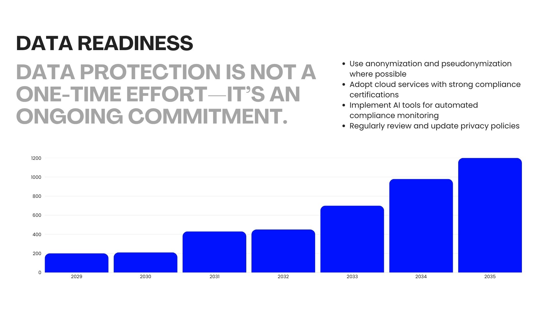
“Data protection is not a one-time effort—it’s an ongoing commitment.”

Why I stopped waiting for real patient data and started generating my own — a working guide to Synthea, Parquet, and the data stack I actually use.

Why I’m writing this

I’ve lost count of how many times I’ve sat in a meeting — or these days, a Teams call — and watched a genuinely good idea die because nobody could get the data to test it.

A clinician sketches out a readmission risk model. A vendor demos a slick FHIR-based mobile app. Someone on my team proposes a lakehouse migration that would actually fix the reporting chaos. Every single time, the conversation ends the same way:

“This looks promising. Can we try it on our actual patients first?”
“Sure. We just need to get data access approved.”

And then six months disappear.

The hardest problem I keep running into in healthcare data isn’t model accuracy, or architecture, or security. It’s access. Real patient data is locked behind compliance walls — for very good reasons — and that means most of us who want to learn, prototype, teach, or just demo something can’t actually get the dataset we need to do the work.

For a long time, I tried to work around this. Anonymized exports that took weeks to approve. Toy datasets that didn’t behave anything like real records. Notebooks built on the Titanic CSV, pretending the lessons would somehow transfer to ICU patients. None of it really worked.

At some point I stopped fighting the wall and started simulating what was behind it. This post is what I wish someone had handed me three years ago: a practical walkthrough of how I use Synthea to generate realistic patient populations, and how I turn that output into Parquet so the rest of my data stack can actually consume it.

Here’s the path I’ll take you through:

1. The access problem, from someone who has lived inside it
2. Why I think Synthea, specifically, is worth your time
3. Getting it installed and generating your first population
4. Converting CSV to Parquet — four ways, depending on how big you’re going
5. Sanity-checking the output
6. What I’m planning to build on top of this dataset next

If you’re a data engineer, ML practitioner, healthcare developer, or just curious about how synthetic data works in a regulated industry, this is for you.

Part 1 — The problem I kept hitting

The compliance wall is real

Healthcare data is governed by HIPAA in the US, GDPR in Europe, and here in the UAE by DHA and ADHICS frameworks (with equivalents almost everywhere else). The rules differ in detail but agree on the basics: Protected Health Information cannot leave controlled environments, cannot be shared with vendors without a Business Associate Agreement or equivalent, and cannot be used for purposes the patient didn’t consent to.

I’ve been on both sides of that wall. I understand exactly why it exists, and I’m not arguing against it. But the practical consequence — even with the best intentions on every side — is that getting access to real data for a POC looks something like this:

• An IRB or ethics committee review
• A data use agreement
• A de-identification pipeline (which itself is a project)
• A network-isolated environment with no internet egress
• Months of waiting

A developer trying to learn FHIR cannot wait for that. A startup pitching an AI triage tool cannot wait for that. A data engineering team prototyping a lakehouse cannot wait for that. I couldn’t wait for that — not for a learning project, not for a side experiment, not for the kind of “let me just try something” exploration that makes you better at this work.

Why “just anonymize it” never solved it for me

Every time I’ve raised the access problem with someone, the suggestion comes back: anonymize the data. I’ve tried this. Twice it actually helped. Most of the time, two things kill the approach:

1. It’s still treated as real data. Re-identification attacks are well-documented — the Netflix Prize, the Massachusetts governor’s medical records, the AOL search logs — and most legal teams (correctly) treat anonymized health data with caution. The wall gets shorter, not removed.
2. Strong anonymization destroys the signal. k-anonymity or differential privacy aggressive enough to satisfy a privacy officer is usually aggressive enough to flatten the rare, edge-case, long-tail behaviour that ML models actually need to learn from.

You end up with data you can’t fully share and can’t fully use. The worst of both worlds.

What synthetic data changed for me

I came to Synthea reluctantly. I’d assumed synthetic data would be too sanitised to be useful — generic enough to compile, useless to learn from.

What changed my mind was watching it generate a single patient and trace her through her entire life: a normal childhood, gestational diabetes during a pregnancy, gradual progression to Type 2 diabetes a decade later, the cardiovascular complications that statistically follow, the end-of-life encounter that looked exactly like the ones I’d seen in real charts. The individual person was fabricated. The clinical pattern was correct.

That was the moment I realised: for everything that isn’t actual clinical decision support, this is enough. For learning, for prototyping, for teaching teammates, for showing a stakeholder what a feature would look like, for benchmarking a Spark job — this is more than enough.

The dataset I needed wasn’t real data. It was data that behaves like real data, which I’m allowed to share, query, break, and rebuild.

What I look for in a synthetic dataset

After working with a few of these, my checklist comes down to four things:

• Statistically realistic — distributions, correlations, and edge cases mirror reality, even if the individual records are fabricated
• Schema-faithful — if production uses FHIR R4, my synthetic data should too, so the code I write actually transfers
• Reproducible — same seed, same patients, so I can debug
• Free of restrictions — Apache or MIT licensed, no usage limits, shareable in a public Git repo or a blog post like this one

Synthea ticks all four boxes, which is why I keep coming back to it.

Part 2 — What Synthea actually is

Synthea is an open-source patient population simulator from MITRE Corporation, released under Apache 2.0. It models complete patient lives — birth, demographics, the development and progression of diseases, encounters with the healthcare system, medications, labs, procedures, and eventually death — using a modular rules engine grounded in real epidemiology research.

You give it a state, a city, and a population size. It simulates that many people from birth to present day and emits the full medical history of each one. The default exporters cover:

• HL7 FHIR (R4, STU3, DSTU2) — the standard healthcare API format
• Bulk FHIR in NDJSON
• CSV — flat tables, easy to load anywhere
• C-CDA — older clinical document standard
• CPCDS — claims data format

The Springer collection Synthetic Data for Health is a useful academic companion if you want to see how this kind of data is being used in published research.

One warning before you start

The synthetichealth/synthea image on Docker Hub exists, but it is over nine years old and based on an older Ruby implementation that has been superseded. I learned this the embarrassing way after wondering for half an hour why the flags in the docs didn’t match what was working. The current Synthea is Java-based and lives on GitHub. Don’t pull that image. Build from source, or wrap the current Java version in your own thin Dockerfile — I’ll show one below.

Part 3 — Generating my first patient population

Prerequisites

• Java JDK 17 or 25 (LTS releases). I’ve hit weird issues on non-LTS versions, so I just stick with these.
• Git.
• About 1 GB of free disk for a 1,000-patient run with all exporters on.

Clone and build

git clone https://github.com/synthetichealth/synthea.git
cd synthea
./gradlew build check test

The first build pulls dependencies and runs the test suite — give it 5–10 minutes the first time. On Windows replace ./gradlew with gradlew.bat.

My smoke test before any real run

Before I commit to generating a large population, I always run a tiny smoke test:

./run_synthea -p 10

This generates 10 patients using Massachusetts demographics (the default) and drops FHIR R4 bundles into ./output/fhir/. Open one of those JSON files — you’ll see a complete patient bundle: demographics, encounters, observations, medications, conditions, the lot. If that looks right, the build is healthy and I move on.

The real run, with CSV enabled

For everything analytics-related, I want CSV (and then Parquet), not FHIR JSON. By default, Synthea only emits FHIR. You turn CSV on either by editing src/main/resources/synthea.properties or by overriding on the command line. I prefer the command line because it leaves the defaults clean:

./run_synthea \
  -s 42 \
  -p 1000 \
  --exporter.csv.export=true \
  --exporter.fhir.export=false \
  --exporter.hospital.fhir.export=false \
  --exporter.practitioner.fhir.export=false \
  Massachusetts

What each flag does:

After a few minutes I get files in ./output/csv/:

allergies.csv
careplans.csv
claims.csv
claims_transactions.csv
conditions.csv
devices.csv
encounters.csv
imaging_studies.csv
immunizations.csv
medications.csv
observations.csv      ← this one gets big fast
organizations.csv
patients.csv
payer_transitions.csv
payers.csv
procedures.csv
providers.csv
supplies.csv

That’s 18 tables of a fully relational synthetic EHR. patients.csv is the dimension. encounters.csv is the spine. Everything else (observations, conditions, medications, etc.) is keyed by PATIENT and ENCOUNTER. The first time I joined them in a notebook and got back a coherent patient timeline, I genuinely smiled.

Variations I reach for

# Specific city
./run_synthea -p 500 Massachusetts Boston

# Just the elderly — useful for cardiac / dementia / fall-risk work
./run_synthea -p 200 -a 65-95

# Just men, in Texas, into a custom output directory
./run_synthea -g M -p 1000 --exporter.baseDirectory="./output_tx/" Texas

# Larger, fixed seed so two teammates generate identical data
./run_synthea -s 12345 -p 10000 Massachusetts

Run ./run_synthea -h for the full option list. I keep a little shell alias around the seeded 1,000-patient Massachusetts run because it’s my default sandbox.

A current Dockerfile, since the official one is stale

I want my generation step to be reproducible across machines, so I wrap it in Docker. Here’s the minimal Dockerfile I use — save it as Dockerfile:

FROM eclipse-temurin:17-jdk AS build
WORKDIR /synthea
RUN apt-get update && apt-get install -y git && \
    git clone https://github.com/synthetichealth/synthea.git . && \
    ./gradlew build -x test

FROM eclipse-temurin:17-jre
WORKDIR /synthea
COPY --from=build /synthea /synthea
ENTRYPOINT ["./run_synthea"]

Build and run:

docker build -t synthea-current .
docker run --rm -v "$(pwd)/output:/synthea/output" synthea-current \
  -s 42 -p 1000 \
  --exporter.csv.export=true \
  --exporter.fhir.export=false \
  Massachusetts

This gives me a stable image I can hand to colleagues without the “did you install the right JDK?” conversation.

ER Diagram for Dataset

Part 4 — Why I move everything to Parquet, and how

CSV is fine for an initial look. It is not fine for analytics at any real scale. The first time I tried to filter observations.csv in pandas without first parsing dates, I sat watching a notebook hang for a few minutes before I killed it. That was when I learned to move to Parquet as the very first step of any Synthea pipeline.

What Parquet gives me over CSV

• Columnar. A query that touches three columns reads only those three columns from disk. Huge speedup on wide tables like observations.
• Compressed. Snappy or Zstd typically shrinks Synthea CSV by 5–10×.
• Typed. Schema is embedded in the file. No more pd.read_csv(..., dtype={...}) boilerplate, no more dates parsed as strings on every load.
• Partition-friendly. Split by year, state, encounter type — engines will prune partitions automatically.
• Native to the modern stack. Microsoft Fabric Lakehouses, Databricks, Snowflake’s external tables, BigQuery’s external tables, DuckDB, Polars, Spark — they all speak Parquet first.

I’ll show you four ways I’ve used to convert, from simplest to most scalable. Pick the one that matches your situation.

Approach A — Pandas + PyArrow (what I use on a laptop)

Fine for datasets up to a few GB.

# requirements: pandas>=2.0, pyarrow>=14.0
from pathlib import Path
import pandas as pd

CSV_DIR = Path("output/csv")
PARQUET_DIR = Path("output/parquet")
PARQUET_DIR.mkdir(parents=True, exist_ok=True)

# Date columns I parse up front, per the Synthea CSV schema.
# Doing this here means the Parquet files have proper timestamp types,
# not strings I'll have to re-cast every time I open them.
DATE_COLS = {
    "patients":      ["BIRTHDATE", "DEATHDATE"],
    "encounters":    ["START", "STOP"],
    "conditions":    ["START", "STOP"],
    "medications":   ["START", "STOP"],
    "observations":  ["DATE"],
    "procedures":    ["START", "STOP"],
    "immunizations": ["DATE"],
    "allergies":     ["START", "STOP"],
    "careplans":     ["START", "STOP"],
    "imaging_studies": ["DATE"],
    "devices":       ["START", "STOP"],
    "supplies":      ["DATE"],
    "payer_transitions": ["START_DATE", "END_DATE"],
    "claims":        ["CURRENTILLNESSDATE", "SERVICEDATE"],
    "claims_transactions": ["FROMDATE", "TODATE"],
}

for csv_path in sorted(CSV_DIR.glob("*.csv")):
    table = csv_path.stem
    print(f"Converting {table}...")

    df = pd.read_csv(
        csv_path,
        parse_dates=DATE_COLS.get(table, []),
        low_memory=False,
    )

    out_path = PARQUET_DIR / f"{table}.parquet"
    df.to_parquet(
        out_path,
        engine="pyarrow",
        compression="snappy",
        index=False,
    )
    print(f"  -> {out_path}  ({out_path.stat().st_size / 1024:.1f} KB)")

For observations — the one big table that always pushed me into memory pressure — I switch to a chunked writer:

import pyarrow as pa
import pyarrow.parquet as pq

writer = None
for chunk in pd.read_csv(CSV_DIR / "observations.csv",
                         parse_dates=["DATE"],
                         chunksize=200_000,
                         low_memory=False):
    table = pa.Table.from_pandas(chunk, preserve_index=False)
    if writer is None:
        writer = pq.ParquetWriter(PARQUET_DIR / "observations.parquet",
                                  table.schema, compression="snappy")
    writer.write_table(table)
if writer:
    writer.close()

Approach B — Polars (my favourite for laptop work now)

Once I discovered Polars’ streaming pipeline, I mostly stopped reaching for pandas for this kind of work. The whole conversion becomes two lines per file and runs without loading the data into RAM:

# requirements: polars>=0.20
import polars as pl
from pathlib import Path

CSV_DIR = Path("output/csv")
PARQUET_DIR = Path("output/parquet")
PARQUET_DIR.mkdir(parents=True, exist_ok=True)

for csv_path in sorted(CSV_DIR.glob("*.csv")):
    out_path = PARQUET_DIR / f"{csv_path.stem}.parquet"
    (
        pl.scan_csv(csv_path, try_parse_dates=True, infer_schema_length=10_000)
          .sink_parquet(out_path, compression="snappy")
    )
    print(f"{csv_path.name} -> {out_path.name}")

scan_csv + sink_parquet is a true streaming pipeline. Polars reads CSV in batches and writes Parquet in batches without ever holding the whole frame in memory. The first time I ran this on a 10,000-patient generation it finished while I was still preparing for it to take a while.

Approach C — PySpark (when I’m going to the lakehouse)

When I scale up — multiple states, hundreds of thousands of patients, partitioning by year — this is what I use. It also drops cleanly into Microsoft Fabric, Databricks, or EMR if that’s where the work is going.

# requirements: pyspark>=3.5
from pyspark.sql import SparkSession
from pyspark.sql.functions import col, year

spark = (
    SparkSession.builder
    .appName("synthea-csv-to-parquet")
    .config("spark.sql.session.timeZone", "UTC")
    .getOrCreate()
)

CSV_DIR = "output/csv"
PARQUET_DIR = "output/parquet"

tables = [
    "patients", "encounters", "observations", "conditions",
    "medications", "procedures", "immunizations", "allergies",
    "careplans", "providers", "organizations", "payers",
    "payer_transitions", "imaging_studies", "devices",
    "supplies", "claims", "claims_transactions",
]

for t in tables:
    df = (
        spark.read
             .option("header", "true")
             .option("inferSchema", "true")
             .csv(f"{CSV_DIR}/{t}.csv")
    )

    # I partition the big, time-series tables by year for fast pruning later.
    if t == "encounters":
        df = df.withColumn("year", year(col("START")))
        df.write.mode("overwrite").partitionBy("year").parquet(f"{PARQUET_DIR}/{t}")
    elif t == "observations":
        df = df.withColumn("year", year(col("DATE")))
        df.write.mode("overwrite").partitionBy("year").parquet(f"{PARQUET_DIR}/{t}")
    else:
        df.write.mode("overwrite").parquet(f"{PARQUET_DIR}/{t}")

    print(f"Wrote {t}")

spark.stop()

Two things I’ve learned the hard way with this version:

• inferSchema is convenient but slow on huge files. For production, I define schemas explicitly.
• Partitioning encounters and observations by year is the single highest-leverage change I can make for query performance. Most clinical questions are time-bounded.

The output is a folder per table, not a single file — that’s the standard lakehouse layout, and Fabric / Databricks expect it.

Approach D — DuckDB (when I just want SQL)

Sometimes I don’t want to set up a Python environment at all. DuckDB is my answer:

-- duckdb shell, run from inside the output/ directory
INSTALL parquet; LOAD parquet;

COPY (SELECT * FROM read_csv_auto('csv/patients.csv'))
  TO 'parquet/patients.parquet' (FORMAT PARQUET, COMPRESSION ZSTD);

COPY (SELECT * FROM read_csv_auto('csv/encounters.csv'))
  TO 'parquet/encounters.parquet' (FORMAT PARQUET, COMPRESSION ZSTD);

-- repeat per table, or wrap in a shell loop

DuckDB also lets me query the CSV directly without converting, which is what I do when I’m just exploring:

SELECT GENDER, COUNT(*) FROM read_csv_auto('csv/patients.csv') GROUP BY 1;

Part 5 — How I sanity-check the output

Generation finishes, files exist, Parquet is written. But is the data actually right? I always run two quick checks before I trust the dataset for anything else.

import polars as pl

patients = pl.read_parquet("output/parquet/patients.parquet")
encounters = pl.read_parquet("output/parquet/encounters.parquet")

# 1. Basic counts and shape
print("Patients:", patients.height)
print("Encounters:", encounters.height)
print("Encounters per patient:", encounters.height / patients.height)

# 2. Demographic distribution — should roughly match the state I picked
print(patients.group_by("GENDER").len())
print(patients.group_by("RACE").len().sort("len", descending=True))

For a 1,000-patient Massachusetts run with the defaults I should see a roughly even gender split, the majority race recorded as “white” (reflecting MA demographics), and somewhere in the 50–80 encounters-per-patient range across a lifetime.

If those numbers look wildly off, something went wrong — usually it’s that a flag silently disabled an exporter, or my seed happened to produce an unusual cohort. Either way, I rerun before I waste time downstream.

Part 6 — What I’m planning to build on this

Now that I have a Synthea Parquet dataset I can rebuild on demand, here’s where this series is going next:

Automated relationship discovery. Microsoft’s tutorial on discovering relationships in the Synthea dataset is a great showcase of Semantic Link / SemPy. You feed it the Synthea CSVs and it figures out, automatically, that encounters resolves a many-to-many between patients and providers, that observations hangs off encounters, and so on. This is genuinely useful any time I inherit a data model with no documentation — and Synthea is the perfect teaching set for it because I already know the answers. My next post will do the same thing on the Parquet output using Polars and DuckDB instead of pandas.

Lakehouse modelling. Bronze / silver / gold layering on Synthea, with conformed dimensions for patient, provider, and encounter, and a wide observations fact. Synthea is small enough to iterate on quickly but rich enough to model properly.

Clinical feature engineering. Rolling vitals windows, comorbidity flags, medication adherence proxies — the features that go into readmission, sepsis, or no-show prediction models.

LLM and RAG patterns. Synthea also emits FHIR JSON and (with a flag) clinical-style notes. I want to index them in a vector store, build a RAG pipeline that answers questions about a patient’s history, evaluate hallucination rates — all on data I can publish openly.

Time-series forecasting. Observations are time-stamped vitals. A clean practice ground for Prophet, ARIMA, or a small transformer.

Differential privacy experiments. Because the data is already synthetic, I can publish both attack code and defences openly — something I’d never do on real PHI.

TL;DR

If you want to skip everything I wrote and just get to a Parquet dataset:

# 1. Build Synthea
git clone https://github.com/synthetichealth/synthea.git && cd synthea
./gradlew build -x test

# 2. Generate a reproducible 1,000-patient CSV dataset
./run_synthea -s 42 -p 1000 \
  --exporter.csv.export=true \
  --exporter.fhir.export=false \
  Massachusetts

# 3. Convert to Parquet (Polars, streaming)
python -c "
import polars as pl, pathlib
for p in pathlib.Path('output/csv').glob('*.csv'):
    pl.scan_csv(p, try_parse_dates=True, infer_schema_length=10_000) \
      .sink_parquet(f'output/parquet/{p.stem}.parquet', compression='snappy')
"

# 4. Query it from anywhere that speaks Parquet.

That’s the dataset I wish I’d had on day one. No IRB. No DPA. No six-month wait.

In the next post, I’ll load this into a notebook, run automated relationship discovery on it, and start building the silver layer of a proper lakehouse on top. If you want to follow along, generate the dataset now — you’ll be ready when it goes up.

Synthea is © MITRE Corporation, licensed Apache 2.0. The dataset and tooling described here are open source. The patients are not real. The lessons are.